If you’re new to the world of deep learning, you might be overwhelmed by the number of different concepts you come across. But don’t worry; you don’t need to fully understand all the underlying details and the boring mathematics to start working with neural networks. Don’t get me wrong, it’s important to know how things are working behind the scenes, but what I mean is that the best approach is to start applying stuff practically while simultaneously getting an in-depth understanding along the way, one thing at a time.
So today, in this article, we will neural network from scratch in Python using the Keras library. Keras is a Python library that provides a high-level interface to communicate with TensorFlow for implementing neural networks easily. We’ll learn more about it later in the article.
Note: If you want to jump directly to the code, find the notebook with complete source code here.
What Are Neural Networks?
Neural networks, sometimes known as Artificial Neural Networks, are complex models built following the human brain structure. It contains several layers placed one after another, containing a certain number of neurons.
How Many Layers to Use?
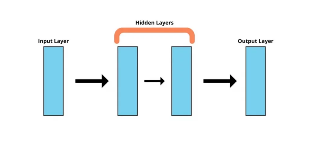
Knowing how many hidden layers to use is essential before creating our model, even if we’re using a high-level interface such as Keras. This highly affects the accuracy metrics and how well your model can make predictions.
The number of layers a neural network contains defines how complex and powerful it is. A greater number of layers means that it will be able to learn more complex parameters. For example, having only a single layer other than the input and output layer will make the network only capable of learning linear relationships.
However, this doesn’t mean that you should add a large number of layers blindly, thinking the model would perform better. There are many other aspects to think about as well, such as overfitting and vanishing gradients. So, it’s recommended to only add the layers that get the job done.
Training a Neural Network in Python
Training a neural network model can be a bit of a mess and requires a solid understanding of all the concepts such as the activation functions, neuron bias, gradient descent, and so on. But thanks to Keras, we will not have to implement all of this ourselves. Rather, we will use the Keras API and use its built-in functions. Let’s start with it in a step-by-step manner.
Actually, before we hit it off, make sure you have a Google Colab or Jupyter Notebook set up with Python 3.6 or later running on it. Hop on here if you don’t know how to set it up. That’s all you need to have; I’ll explain the other stuff along the way.
1. Loading Data & Importing Libraries
We’ll be using the Pima Indians Diabetes dataset for demonstration purposes since it’s easier for beginners to use as all the input variables are numerical. The dataset contains the data about sugar patients, and we will be using it to predict if a particular patient suffers from diabetes or not. Download the dataset and place it locally on your computer. More details about the dataset and the columns can be found here.
Next, import the required libraries and the dataset as shown below. Numpy and pandas are to import and manipulate the data while Keras is to create our model:
| import pandas as pdfrom numpy import loadtxtfrom tensorflow.keras.models import Sequentialfrom tensorflow.keras.layers import Dense |
That’s pretty much everything we need to use our dataset and train the neural network.
Let’s proceed with loading the dataset and storing it in separate training and target feature arrays. We will use the loadtxt() method of numpy we just imported to first read the data and then split it into separate arrays for feature and target variables:
| dataset = loadtxt(‘Desktop/pima-indians-diabetes.csv’, delimiter=’,’) X = dataset[:,0:8]y = dataset[:,8] |
Wonder how the variables look? Let’s take a look by printing the X array:
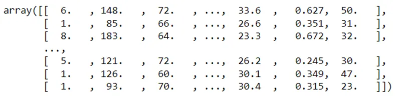
As you can see, the X array holds a list of lists, with each of the inner lists corresponding to a training example in the form of a vector. There will be exactly eight numbers in an array since the dataset contains eight different variables.
Similarly, if you try to view the y array, you will see that the vectors have only 1 number in them since there’s only a single target variable, which will be either 1 or 0 (Positive and Negative class).
Next up, we also need to split our data for training and testing. This is to ensure that the data we use for testing our model is not the same that we used in the training. Otherwise, it can lead to misleading results since the model has already ‘seen’ the data. We’ll leave roughly 30% of the data for testing and use the rest for training.
| X_train = X[:568]y_train = y[:568] X_test = X[568:]y_test = y[568:] |
That’s it. Let’s move on to defining our Keras model now.
2. Defining the Model
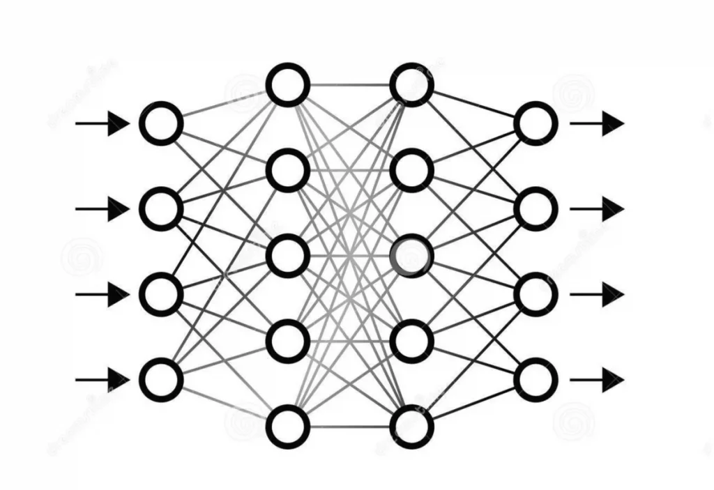
We discussed how layers are used in the architecture of neural networks above. So here, we’re going to do just that, using Keras. The way we do this is to make separate layers and place them sequentially, one after the other. This is called a sequential model.
First things first, we have to make sure the input layer can handle our training vectors. We have to set the shape of the first layer according to the shape of our X variable that we defined above. Since the size of each array in the training data was eight, the size of the input layer will be eight too.
Next up, we need to decide how many hidden layers to add. But wait, how do we know how many layers we need? Well, as mentioned before, that’s a whole different process and currently outside the scope of this article. Right now, you just need to ensure they’re enough to capture the dataset details but not too many to overfit the data.
Therefore, since the data is not too complex, but we don’t just want our model to spot linear relationships, we will use a total of four layers. We generally don’t count the input layer as a layer, with three hidden and one output layer. We will use the ReLU activation function in the hidden layers and sigmoid in the output layer since we want to classify the cases as 0 or 1. Sigmoid basically turns probabilities into binary outputs by thresholding them at 0.5. More on it here.
So, here’s a quick summary of how we’re gonna build the model architecture:
- Define three hidden fully-connected layers and one output layer
- Make sure the first layer expects vectors of shape (,8)
- Use ReLU in the hidden layers and Sigmoid in the output layer
Let’s see how we can do this in Python.
| model = Sequential()model.add(Dense(10, input_shape=(8,), activation=’relu’))model.add(Dense(8, activation=’relu’))model.add(Dense(8, activation=’relu’))model.add(Dense(1, activation=’sigmoid’)) |
That’s it. Run this cell, and we’re done with the architecture. Let’s move on to compiling the model now.
3. Compiling & Fitting the Model
Before we move on to fitting the model and training it using the dataset we imported, we have to compile the model. The process basically involves the backend, TensorFlow in this case, deciding how to represent the model to train and make predictions. This is done while keeping the underlying hardware and software in mind. However, since we’re on Jupyter/Colab, we don’t need to worry about it.
We will use to compile method provided by Keras to do the deed and specify the loss and optimizer we will use to train our model. For loss, we will use cross-entropy, and for the optimizer, we’ll use Adam. Why use these? Well, cross-entropy is a proven loss function that provides excellent results in the domain of binary classification and Adam because it works well with most of the generic deep learning models, basically a go-to for most deep learning engineers.
| model.compile(loss=’binary_crossentropy’, optimizer=’adam’, metrics=[‘accuracy’]) |
If you wish to calculate other accuracy metrics, you can also pass them along with accuracy in the list at the end. That’s actually it for compiling—the beauty of Keras.
To fit the model. We need some more information, such as epochs and batch size. Epoch will determine the number of passes the model will make through the training dataset. And batch size tells us the chunks in which we’re going to divide our training set for each epoch. If you don’t know about these parameters, you read my previous article, where I talked about them in detail here.
Other than these parameters, we need to pass the training data. This will consist of the arrays we initialized towards the start of the article. Let’s pass all this data to start the model training:
| model.fit(X, y, epochs=20, batch_size=10) |
The values for these parameters can be changed depending upon the use case. A complex dataset might require a much bigger number of epochs. But 50 works for this case just fine since we didn’t have much data to start with, but it’s also not very complex. Also, it’s worth mentioning that the greater number of epochs you define, the more time it’ll take for the model to train – since it has to pass the complete training data through the model more times then, right?
Let’s run the cell and wait for the training to complete.
4. Evaluating the Model
Let’s now evaluate our model and see how well it performs classification. To make the evaluation, we will use the evaluate() provided by Keras and pass in the testing and training arrays. Make sure you don’t pass in the same arrays as you did while training the model. Otherwise, you may get excellent results, but in reality, your model will not perform as well on the new ‘unseen’ data.
Here’s how we can evaluate the model.
| i, acc = model.evaluate(X_test, y_test)print(‘Accuracy: %.2f’ % (acc*100)) |
The function outputs two variables, accuracy and loss. We can also print the loss just like accuracy, but we don’t need it for now. Let’s run the cell and see what we get:

Amazing! While 71% is certainly not a great number, it’s definitely a very decent number to start with, especially considering how we just trained the model for demonstration purposes and the tiny amount of data we had. If you put more effort into choosing the suitable parameters, such as the number of layers, activation function, and so on, you can easily get an accuracy of above 90%. And don’t forget this model was trained on just over 500 samples!
That’s all! Note that you can also use this model to make predictions on new unseen data using the Keras’ predict()function. Just pass in the data as a vector having the correct dimension, and the model will tell you whether the sample belongs to class 0 or 1.
Let’s wrap things up in the next section.
Conclusion
Neural networks are making considerable strides in the world of artificial intelligence. Given their ability to train themselves and do feature extraction by themselves, they’ve been gaining a lot of popularity, not to mention their complex structure, which is able to capture the most minor of the details in a dataset.
However, just how well they perform, they’re equally challenging to understand. It’s hard for a newbie to develop a neural network from scratch without understanding the ocean of maths under the surface. But fortunately, we have libraries like Keras that make it very easy for us to implement neural networks while knowing just their basics.
Throughout the article, we’ve seen how Keras handles everything under the hood and lets us build neural networks quickly. More so, this doesn’t come at the expense of customizability, and we can still tweak the models according to our needs.
